
Measures of Inequality: The Gini-Coefficient
- 29. aug. 2016
- 3 min læsning
The Lorenz-curve
The Gini-coefficient is probably the most used method of measuring inequality. The Gini-coefficient shows how a resource is distributed in a population.
The Gini-coefficient is built upon the Lorenz-curve and it gives a visual picture of how a given resource (in this case income) is distributed in a given population. The Lorenz-curve is in other words a visual presentation of the accumulated distribution function. In the following the Lorenz-curve is thus a graph where the accumulated share of the total income is plotted against the accumulated percentage of the population arranged in increasing order. Thus the Lorenz-curve shows how a ranked and accumulated distribution is distributed. It is often given in groups (eg. deciles of a population). The extent to which the curve arches below the diagonal that represents perfect equality therefore indicates the degree of inequality in the distribution of income.
Firstly the population is arranged in order starting from the lowest and ending with the highest. The Lorenz-curve thus plots the share of the population against the share of the total income of the same population. This is shown in figure 1:
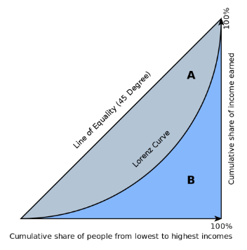
Figure 1
Suppose that there are N individuals whose incomes are denoted yi where i = 1, … N and that the incomes are arranged in increasing order so y1 ≤ … ≤ yi ≤ yn. This means that the first k individuals in the order of incomes have the cumulated income:
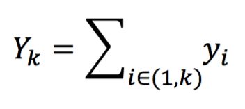
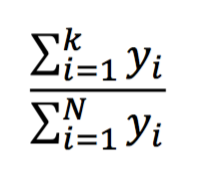
In other words: The lorenz-curve shows the relationship between the share of individuals who have an income that is lower or equal to a specific amount and the share of the total income these individuals have. The share of individuals with an income which is lower than income number k in the order is then: k/N. The corresponding share of the total income is then:
We can illustrate this by using an example:
If k = 1 the share of individuals with a lower income than income number k will be: 1/N and these individuals’ share of the total income will be y1/Nȳ, where ȳ is the middle-income. We use the accumulated percentages converted to decimal figures, which means that G∈[0;1], where G is the Gini-coefficient.
In a system of coordinates with the Lorenz-curve there is an 45° diagonal from origin to the point (1,1). The slope is equal to 1 and its form is thus: P(x) = x, where P is the distribution in percent of the total income and x is the share of the population in percent. This line represents perfect equality. The area Ap under P down to the x-axis in [0,1] is thus:

The curve will always lie under the diagonal expect when yi = ȳ. The Lorenz-curve has two extremes:
Perfect inequality where one individual owns 100% of the total income and the rest owns nothing. When N owns all of the income then for every k < N. In this case the curve will crawl along the x-axis to the right-hand corner and then up to (1,1)
Perfect equality. Everyone has the same income: yi = ȳ. The share of the total income for all k is and is equal to the corresponding share of individuals. The lorenz-curve is, in this case, equal to the diagonal.
The closer the lorenz-curve is to the diagonal the more equal the population is.
This means that the Lorenz-curve L(x) is continuous in [0,1], L(0) = 0, L(1) = 1, L(x) increases in the interval [0,1] and L’(x) is not decreasing in the interval [0,1] – though it can be linear. The Lorenz-curve is plotted as a summation curve.
It is important to be aware of what the Lorenz-curve is in order to calculate the Gini-coefficient. The Gini-coefficient summarises the degree of inequality in one number. It shows the difference between the current income distribution and a perfectly equal income distribution. This is where the Lorenz-curve becomes interesting. In order to calculate the Gini-coefficient one has to finds the coefficient between the actual inequality and the minimal inequality and the difference between the maximum inequality and the minimal inequality. This means that one has to find the coefficient between the area under the diagonal and the Lorenz-curve and the area that makes up the whole area under the diagonal. This can be done in a number of different ways.
Looking af Figure1 we can conclude that:

Kommentarer